Urban-rural divide in foodborne illness in China: what can we learn from the socioeconomic factors?

Food supply and safety are major global public health issues.¹ With a population of 1.39 billion, one of China’s greatest challenges is to ensure the safety of its food supply chain. The Chinese government has made progress in establishing a quality regulatory system designed to promote quality food safety standards across the country.² For example, China’s Food Safety Law of 2015 was wide ranging in scope and imposed strict controls over the production, management, and distribution of food. While it might be too early to determine the overall effectiveness of the 2015 law, some early studies have shown that food safety continues to be a problem in China. A study by Yasuda³ argues that Chinese regulators face a fundamental policy challenge related to China’s massive production system, unwieldy bureaucracy, and geographic size. Specifically, Yasuda³ argues that as Chinese regulators attempt to build an integrated national regulatory regime, often they have had to make difficult trade-offs between cost and policy designs which reflect the interests of certain stakeholders over others. Therefore, China’s food safety problem must be understood as a result of the scale of its food production system as well as the politics of its regulatory processes. A study by Ortega et. al.⁴ explores Chinese food safety issues by analysing selected incidents within the Chinese agricultural marketing system and argues that food safety issues arise from problems of asymmetric information in which consumers do not have complete or even partial information about the safety of the food they are purchasing and do not trust private or government inspections. Profit-seeking behavior in the presence of asymmetric information combined with a lack of confidence in the quality of food served in the marketplace led to practices that have worsened food safety across the country.

Other studies find that a major cause of the food safety issue is the disconnect between China’s rural and urban food safety systems. Liu and McGuire⁵ argues that unlike their urban counterparts where district-level administrators exercise strict control over food safety standards, rural food safety bodies are often weak and unable to enforce reliable food safety standards. This weakness may be the result of limited government financial support which prevents them from hiring the highly trained and educated personnel employed in urban areas. Furthermore, inadequate funding forces them to rely on “extra-budgetary” fees to help cover expenditures which in turn open the door to corruption and bribery.

The disparity in consumption and income between urban and rural areas in China is a serious issue. In this study, socioeconomic factors associated with urban–rural disparity in the number of color TVs per 100 households, refrigerators per 100 households, real food consumption expenditure per capita and real income per capita in China are explored to determine how much of the urban–rural divide is related to foodborne illness while holding constant socioeconomic factors that capture media influence, economic development, and agricultural production factors. To achieve this objective, the current study estimates several panel data models of foodborne illness in China in order to make causal inferences while controlling for unmeasured confounders.

Methods

This study revisits Holtkamp, Liu, and McGuire⁶ to examine how socioeconomic factors influence food safety in China. Where Holtkamp et. al.⁶ used China media data on foodborne incidents and a Tobit⁷ random effects model, this study uses panel data collected from various issues of the China Health Statistical Yearbook⁸ and the China Statistical Yearbook.⁹ Linear and nonlinear panel data models are estimated to explore how variations in socioeconomic factors in and across urban and rural areas help to explain the incidents of foodborne illness across Chinese provinces from 2011 to 2018.

Model specification

“The fundamental problem for statistical analysis in the social sciences has been how to make causal inferences from nonexperimental data¹⁰ and a widespread consensus has long been reached that the best kind of nonexperimental data for making causal inferences is longitudinal data, i.e. panel data. Economists have distinguished between fixed effects and random effects models and have developed several novel estimation methods for handling various elaborations of these models.”¹¹

The model in this study is specified as follows.

$$y_{\text{it}} = \mathbf{x}_{\mathbf{\text{it}}}\boldsymbol{\beta} +c_{i} + \epsilon_{\text{it}}\hspace{10mm}(1)$$

where i = 1, 2, . . . , 26 represent the provinces in China including Beijing, Tianjin, Hebei, Shanxi, Liaoning, Jilin, Heilongjiang, Shanghai, Jiangsu, Zhejiang, Anhui, Fujian, Jiangxi, Shandong, Henan, Hubei, Hunan, Guangdong, Guangxi, Hainan, Chongqing, Sichuan, Guizhou, Yunnan, Shaanxi, and Gansu, but excluding Tibet, Xinjiang, Ningxia, Qinghai and Inner Mongolia, due to the limited availability of the data. t = 2011, 2012, …, 2018. $y_{\text{it}}$ is the number of foodborne incidents per capita or the number of foodborne patients per capita. $\mathbf{x_{it}}$ is a $(1\times 19)$ vector of independent variables. $\boldsymbol{\beta}$ is a $(19\times 1)$ vector of regression coefficients. $c_{i}$ is the time constant unobserved effects or the heterogeneity effects. $\epsilon_{\text{it}}$ is an idiosyncratic standard normally-distributed error term. Initial check on the correlation coefficients among the 19 covariates indicates no multicollinearity using this more elaborate model. These 19 independent variables capture four aspects of the food safety issues that have all been addressed in recent food safety studies.^6,12–24 This study adds to the literature by investigating these variables jointly.

Dependent variables

Table 1 describes that the dependent variable foodborne illness is measured either by the number of foodborne incidents per capita (inci_pc) or the number of foodborne patients per capita (pa_pc). Larger provinces may have larger numbers of foodborne incidents or patients, so it is important to take into account the overall population of each province.

Independent variables

Table 1 also describes the independent variables and categorizes them into four types of socioeconomic factors.

Media influence

One study conducted by using the U.S. Food Safety Surveys shows that media can help monitor and expose food safety issues as increased media attention to food safety issues may raise consumers’ awareness of food safety hazards and increase vigilance in proper food handling.¹² Scientists and regulators need to understand the complex relationship between the media and their audience if they want to counter scare stories and place the risks and benefits in their proper context.¹³ This study uses log printed copies of newspapers per capita (lnewsp_pc) and log broadband subscribers of internet per capita (lBBS_pc) to measure the media influence which is expected to have negative effects on foodborne illness.

Economic development

It is well understood that sustainable agriculture, economic growth, and enhanced livelihoods allow people to have greater access to safe food.¹⁴ This study measures economic development comprehensively by using the urbanization rate (urbanization), log per capita real gross regional product (lRGRP_pc), share of the primary industry in gross regional product (PrimaryShare), log per capita real government expenditure on medical, health care, and family planning (lRGovhealth_pc), and the log number of residents with access to tap water per capita (lWater_pc). It is expected that they shall have negative effects on foodborne illness.

Agricultural production factors

China has become the world’s largest manufacturer and consumer of fertilizers.¹⁵

“In recent years, China’s fertiliser price has seen a rebound in 2017 and is likely to continue rising in 2018 and the reasons for this development can be found in the rising production costs due to higher raw material prices, larger environmental protection pressure by the government, and the supply-side structural reform, which aims to reduce the number of manufacturers from the market.”¹⁶

This study uses the log of producer price index for chemical fertilizers (lPPICFerti), the log of producer price index for pesticides (lPPIPesti) and the log of consumption of chemical fertilizers in tons per capita (lCCFerti_pc) to measure their ecological effects on foodborne illness. The log of irrigated area of cultivated land in hectares per capita (lIA_pc) is also used and is expected to increase the foodborne illness because the agricultural produce or soil might be contaminated.

Urban-rural divide

Consumer behaviour may differ between urban and rural households due to the urban-rural divide ranging from education inequity to the income gap and poverty. Poverty in China is essentially a rural phenomenon.²⁵ This study selects a few consumer staples such as the log number of colour TVs per 100 urban households (lTVur), log number of color TVs per 100 rural households (lTVru), log number of refrigerators per 100 households in the urban area (lFridgeUr), log number of refrigerators per 100 households in the rural area (lFridgeRu), log per capita real consumption expenditure on food in general in urban (lRfoodCur_gen) and rural areas (lRfoodCru_gen) to measure their individual effects on foodborne illness. The log per capita real annual disposable income of urban households (lRincomepc_ur) and the log per capita real net income of rural households (lRincomepc_ru) are also included to measure their direct income effects on foodborne illness. It is expected that there exists an urban-rural disparity in their impact on foodborne illness. Specifically, consumption of luxury goods such as colour TVs and refrigerators in rural areas may crowd out quality food consumption expenditures, therefore causing more foodborne illness. Higher income in rural areas may improve the situation by reducing the foodborne illness whereas higher income in urban areas may worsen the food safety situation because the risk of food safety issues is high when urban people try more expensive and bizarre food.

Estimation methods

Fixed effects estimation

A linear panel data estimation method removes the unobserved effects $c_{i}$ from the stochastic error term $\epsilon_{\text{it}}$ in Equation (1), implying that the unobserved effects can be arbitrarily related to the observed covariates. One of the key assumptions is to govern the conditional distribution of interest, $D\left( y_{\text{it}} \middle| \mathbf{x}_{\mathbf{\text{it}}},c_{i} \right)$. Often the primary interest is the conditional mean $E\left( y_{\text{it}} \middle| \mathbf{x}_{\mathbf{\text{it}}},c_{i} \right)$. $E\left( y_{\text{it}} \middle| \mathbf{x}_{\mathbf{\text{it}}},c_{i} \right) = \mathbf{x}_{\mathbf{\text{it}}}\boldsymbol{\beta +}c_{i}$ for the fixed effects model. The average partial effects (APE) is derived as

$$\frac{\partial E(y_{t}|\mathbf{x}_{\mathbf{t}},c)}{\partial x_{\text{tj}}}\mathbf{=}\beta_{j}.\hspace{10mm}(2)$$

The APE measures the average change in the unit of y when x increases by one unit.

Random effects estimation

According to the linear panel data estimation method for the random effects, the unobserved effects $c_{i}$ are independent of the covariates in Equation (1). Again, one of the key assumptions is to govern the conditional distribution of interest, $D\left( y_{\text{it}} \middle| \mathbf{x}_{\mathbf{\text{it}}},c_{i} \right)$. Often the primary interest is the conditional mean $E\left( y_{\text{it}} \middle| \mathbf{x}_{\mathbf{\text{it}}} \right)$. For the random effects model, $E\left( y_{\text{it}} \middle| \mathbf{x}_{\mathbf{\text{it}}} \right) = \mathbf{x}_{\mathbf{\text{it}}}\boldsymbol{\beta +}c_{0}$, where ${E\left( c_{i}|\mathbf{x}_{\mathbf{\text{it}}} \right) = c}_{0}$. The average partial effects (APE) is derived as

$$\frac{\partial E(y_{t}|\mathbf{x}_{\mathbf{t}},c)}{\partial x_{\text{tj}}}\mathbf{=}\beta_{j}.\hspace{10mm}(3)$$

The APE measures the average change in the unit of y as x increases by one unit.

Tobit random effects estimation

In some datasets, we do not observe values above or below a certain magnitude, due to a censoring or truncation mechanism. In the presence of censoring/truncation, a dependent variable, y, with constrained and clustered observations at the constraint, creates problems for the linear model. In this study, a significant fraction of the data on the number of foodborne incidents per capita or on the number of foodborne patients per capita has close to zero values. OLS on the complete sample is biased and inconsistent.²⁶ OLS on the unclustered part is also biased and inconsistent.²⁶ The Tobit model,⁷ also called a censored normal regression model, is a nonlinear panel data estimation method. Consider the linear regression model with panel-level random effects,

$$y_{\text{it}}^{*} = \mathbf{x}_{\mathbf{\text{it}}}\boldsymbol{\beta +}\upsilon_{i} + \epsilon_{\text{it}}.\hspace{10mm}(4)$$

The random effects, $\nu_{i}$, are i.i.d., $N(0,\sigma_{\nu}^{2})$, and $\epsilon_{\text{it}}$ are i.i.d. $N(0,\sigma_{\epsilon}^{2})$ independently of $\nu_{i}$. $y_{\text{it}}^{*}$ is not observed because of constraints. $y_{\text{it}}^{*}\sim N\left( \mathbf{x}_{\mathbf{\text{it}}}\boldsymbol{\beta},\sigma^{2} \right)$. If $y_{\text{it}}$ is considered to be left-censored at value 0, it means that

$$\begin{align*} &y_{\text{it}} = y_{\text{it}}^{*} &\text{if } y_{\text{it}}^{*} > 0,\\ &y_{\text{it}} = 0 &\text{if } y_{\text{it}}^{*} \leq 0.\\ \end{align*}$$

For this Tobit model, $E\left( y_{\text{it}} \middle| \mathbf{x}_{\mathbf{\text{it}}} \right) = \Phi(\mathbf{x}_{\mathbf{\text{it}}}\boldsymbol{\beta}/\sigma)\mathbf{x}_{\mathbf{\text{it}}}\boldsymbol{\beta} + \sigma\phi(\mathbf{x}_{\mathbf{\text{it}}}\boldsymbol{\beta}/\sigma)$, where $\Phi$ is the cumulative density function for a standard normal random variable and $\phi$ is the probability density function of a standard normal random variable. The average partial effects (APE) is derived as

$$\frac{\partial E(y_{t}|\mathbf{x}_{\mathbf{t}})}{\partial x_{\text{tj}}} = \beta_{j}\Phi(\frac{\mathbf{x}_{\mathbf{\text{it}}}\boldsymbol{\beta}}{\sigma}).\hspace{20mm}(5)$$

It is also the average change in the unit of y when x increases by one unit.

QMLE for fractional probit model

The Quasi Maximum Likelihood Estimation (QMLE)²⁷ estimates a nonlinear regression model where the dependent variable is bounded between 0 and 1. The standard specification for the unobserved effects (UE) fractional probit model is

$$P(y_{\text{it}}|\mathbf{x}_{\mathbf{\text{it}}},c_{i}) = \Phi(\mathbf{x}_{\mathbf{\text{it}}}\boldsymbol{\beta +}c_{i})\hspace{20mm}(6)$$

where $\Phi$ is a cumulative density function of a standard normal random variable. Papke and Wooldridge²⁷ proposed direct models for the conditional mean of the fractional response that keep the predicted values in the unit interval. Essentially, their pooled QMLE method ignores all serial correlation in estimation and uses cluster-robust standard errors. For fractional probit models, $E\left( y_{\text{it}} \middle| \mathbf{x}_{\mathbf{\text{it}}},c_{i} \right) = \Phi(\mathbf{x}_{\mathbf{\text{it}}}\boldsymbol{\beta +}c_{i})$. The APE is derived as

$$\frac{\partial E(y_{t}|\mathbf{x}_{\mathbf{t}},c)}{\partial x_{\text{tj}}} = \beta_{j}\phi(\mathbf{x}_{\mathbf{t}}\boldsymbol{\beta +}c),\hspace{20mm}(7)$$

which is the average change in probability when x increases by one unit.

GEE for fractional probit model

Papke and Wooldridge²⁸ improved upon the pooled QMLE with panel data by introducing the generalized estimating equations (GEE) approach, which models serial correlation (with a constant structure) to try to improve efficiency and the standard errors are still robust. For fractional probit models, $E\left( y_{\text{it}} \middle| \mathbf{x}_{\mathbf{\text{it}}},c_{i} \right) = \Phi(\mathbf{x}_{\mathbf{\text{it}}}\boldsymbol{\beta +}c_{i})$. The APE is the same as Equation (7), which is the average change in probability when x increases by one unit.

Computation requirements

Stata statistical software is used to write programs to perform all the estimations in this study. Stata programs in Papke and Wooldridge²⁸ are used to prepare the codes to estimate the fractional probit models for this study.

Results

More elaborate models

Table 2 shows the average partial effects of 19 socioeconomic variables on the number of foodborne incidents per capita from eight different models. Table 3 shows the average partial effects of the same 19 socioeconomic variables on the number of foodborne patients per capita from eight different models. Because of the small scale of the dependent variables, this study examines the statistically significant covariates and their implications rather than their numerically small point estimates.

Media influence

Both Tables 2 and 3 illustrate that media exposure from newspapers and the internet may serve as a propaganda tool to expose the incidents of foodborne illness. As a result, food producers are more careful to meet food safety policies which lower the number of foodborne incidents or patients. Using a random effects Tobit model and media data on foodborne illness, Holtkamp et. al.⁶ found significant positive relationships between their dependent variable, log reported incidents per capita, and two independent variables, log total newspaper circulation per capita and log internet users per capita. However, they explain that this might be due to media bias. Chen and Feng¹⁷ compared local independent and government newspaper reports on the food safety scandal of Eleme, the top Online to Offline (O2O) take-out service provider in China, to assess heterogeneity in newspapers’ attitudes before and after Eleme was officially exposed. They showed that before the scandal was exposed, independent newspapers more carefully monitored Eleme’s food safety issue than did the local government newspapers which suggests that marketization or deregulation of newspapers might help improve timely media supervision. Zeng et. al.¹⁸ found that food companies strategically responded after the media disclosed food safety incidents in the food markets, suggesting that the media’s action of exposing food incidents may neither lead to improved competitive resource environments nor foster long-term socially responsible food providers. This may raise a challenging issue for the media on how to arouse public attention while promoting responsible conduct in the food industry.

Economic development

Tables 2 and 3 show that as the Chinese economy develops, urbanization tends to worsen the foodborne illness situation, a result that is consistent with studies by Chen,¹⁹ Holtkamp et. al.,⁶ Ortega et. al.⁴ and others. Chen¹⁹ shows how the serious land degradation which occurs during urbanization has worsened the food safety situation. Chen¹⁹ as well as Holtkamp et. al.⁶ explain that rapid urbanization and the explosive improvement in the standard of living have resulted in the diversification of Chinese food composition. Remarkable income increases have created demands for more animal protein, high-quality vegetables and fruits in addition to subsistence grains, which should lead to a decline in food safety problems. However, the coefficients on the log real gross regional product per capita in Tables 2 and 3 are not statistically significant, though their values are negative. The positive association between the number of foodborne incidents or patients and the share of the agricultural sector in the gross regional product as indicated in column (7) (QMLE estimation) indicates that as more and more land is converted to construction use or use for economic development zones, large crop production might come to rely on the heavy use of synthetic fertilizers posing direct and indirect risks to human health.²⁰ Holtkamp et. al.⁶ finds a negative association between foodborne incidents and government expenditure while He et. al.²¹ finds that at the province level, a positive correlation exists between food safety satisfaction and per capita GDP, per capita food safety fiscal expenditure, and food safety fiscal expenditures. The results in this study differs from He et. al.²¹ for two reasons. First, the dependent variable representing the actual number of the foodborne incidents and patients is based on provincial level data taken from the China Health Statistical Yearbooks⁸ whereas He et. al.²¹ used individual level survey data on food safety satisfaction taken from the Asian Barometer Survey (ABS). Second, this study uses per capita government overall expenditure for medical and health care as an independent variable whereas He et. al.²¹ used fiscal expenditures of general public services to represent food safety fiscal expenditure or per capita food safety fiscal expenditure. More people with access to tap water can help reduce the foodborne illness, but this variable is statistically significant with the right sign only in the Tobit model found in column 3 of Table 2. Government spending on the infrastructure which expands the supply of clean tap water can help reduce the foodborne illness. However, Zhang et. al.²² finds that there are annual reports of incidents of tap water pollution caused by cyanobacteria bloom.

Agricultural production factors

For the production-side factors, this study finds a positive association between foodborne illness and the price of pesticides in the random effects, the fixed effects, and the Tobit models as illustrated in columns 1-3 of Table 2 and in columns 2 and 3 of Table 3. FoodPrint,²⁰ He et. al.,²¹ and Zhang et. al.²² also document the negative effects of the use of fertilizer and pesticide on human health. The log of irrigation shows little statistical significance except for the fixed effects model in column (2) of Tables 2 and 3 where more irrigated land implies more foodborne illness. Zhang et. al.²² argues that crop quality depends on the quantity and quality of irrigation water. The small positive coefficient on the log of irrigated areas of cultivated land could be explained by crop contamination from surface water pollutants. Higher demand for chemical fertilizers is associated with more foodborne illness when the price of chemical fertilizers is accounted for as can be seen from the fixed effects model in column 2 of Table 2. The residue of chemical fertilizers on agricultural produce might account for the negative effects of chemical fertilizers on human health.

Urban-rural divide

The urban and rural variables in this study help to explain the relationship between households’ ownership of some of the electric appliances and foodborne illness. They also illustrate the relationships between household income, food consumption, and foodborne illness. Tables 2 and 3 show that owning more colour TVs either in the urban or rural areas does not have a statistically significant effect on foodborne illness. However, more TVs in urban households could make them more aware of food safety issues and more cautious in their food consumption choices which might account for the smaller number of the foodborne incidents. Since TVs are still considered a luxury good in rural Chinese households, owning a TV could result in more frugal consumption of other items such as food, which could increase the foodborne incidents in rural areas.

The positive coefficients on the number of refrigerators per 100 urban households imply that more fridges are positively associated with increased foodborne illness while fridges in rural households are negatively associated with foodborne illness. Fridges are considered necessities in urban households but are luxuries in rural areas which might result in different and complicated food composition patterns between the two areas.

Higher urban household food consumption expenditure in general is associated with a lower number of foodborne incidents or patients as can be seen in the QMLE estimation in column 7 of Tables 2 and 3, whereas this relationship is found in most model estimations for foodborne incidents involving rural households. However, the more food consumed in rural households is associated with more foodborne illness in terms of number of patients per capita as can be seen in column 7 of Table 3. These mixed results might indicate that, although accelerated urbanization is increasing the demand for high-quality and diverse food products,¹⁹ the growing complexity of the urban and rural food supply chains do not allow us to draw any affirmative conclusion about the relationship between food consumption expenditure in general and foodborne illness.

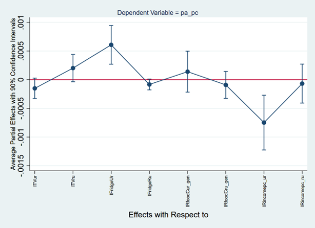
Lastly, coefficients on urban and rural income reveal opposite signs. Higher urban household income is associated with fewer foodborne illness measured by both the number of foodborne incidents and patients, except for column 7 in Table 3, whereas higher rural household income is associated with more foodborne illness as can be seen from both Tables 2 and 3, except for column 7 of Table 3. This might be explained by the fact that the standard of living improves more dramatically in the urban compared to the rural areas. Urban households can afford high-quality safe food whereas the relatively poor rural households have limited choices regarding the quality of their food. However, He et. al.²¹ argues that this is due to the large disparity in amenities between urban and rural development which would include education, income, government resources, and other demographics. In a rural area, residents with agricultural census register are self-sufficient because they can do their own farming and are less dependent on food sold in markets. Food purchased in markets have potential risks due to the aggregation effect of the city which makes the food industry more complicated and increases the consumer distrust of food safety in urban areas. These gaps require governments to respond according to the needs of each area. The characteristics of the average partial effects (APE) of urban and rural variables on the foodborne illness depicted in column 8 of Tables 2 and 3, can also be seen in Figures 1 and 2 where the average partial effects (APE) of only the urban and rural independent variables on the number of foodborne incidents per capita and patients per capita respectively are estimated by the GEE approach. In these two figures, the variables shown on the horizontal axis are the urban and rural independent variables respectively, the dots show the APE estimates and, the vertical lines show the 90% confidence intervals for the APE.

Figure 1.Average partial effects on the number of incidents per capita (inci_pc): generalized estimating equations (GEE).

lTVur = log of number of color TVs per 100 urban households; lTVru = log of number of color TVs per 100 rural households; lFridgeUr = log of number of fridges per 100 urban households; lFridgeRu = log of number of fridges per 100 rural households; lRfoodCur_gen = log of real per capita annual consumption expendiutre on food of urban households, yuan; lRfoodCru_gen = log of real per capita annual consumption expenditure on food of rural households, yuan; lRincomepc_ur = log of per capita real annual (disposable) income of urban households, yuan; lRincomepc_ru = log of per capita real annual (net) income of rural households, yuan

Figure 2.Average partial effects on the number of patients per capita (pa_pc): generalized estimating equations (GEE)

lTVur = log of number of color TVs per 100 urban households; lTVru = log of number of color TVs per 100 rural households; lFridgeUr = log of number of fridges per 100 urban households; lFridgeRu = log of number of fridges per 100 rural households; lRfoodCur_gen = log of real per capita annual consumption expendiutre on food of urban households, yuan; lRfoodCru_gen = log of real per capita annual consumption expenditure on food of rural households, yuan; lRincomepc_ur = log of per capita real annual (disposable) income of urban households, yuan; lRincomepc_ru = log of per capita real annual (net) income of rural households, yuan

Less elaborate models

Because the large number of explanatory variables in the GEE estimation violated the rank condition of the variance and covariance matrix, a less elaborate model with ten independent variables rather than nineteen for the urban equation and similarly for the rural equation are estimated separately using the bootstrap GEE approach. With the dependent variable being the number of foodborne incidents per capita, Figure 3 shows the APE for the urban regression model and Figure 4 shows the APE for the rural regression model. With the dependent variable being the number of foodborne patients per capita, Figure 5 shows the APE for the urban regression model and Figure 6 shows the APE for the rural regression model. The variables shown on the vertical axis are the ten independent variables, the dots show the APE estimates and, the horizontal lines show the 90% confidence intervals for the APE. Figures 3-6 indicate that the food safety problem is intensified by the growth of urbanization and the share of the primary industry, i.e. agriculture, in the gross regional product. The urban and rural variables do not show much of an effect on the foodborne incidents although increasing the number of refrigerators in urban households could increase rather than decrease the number of foodborne incidents or patients as can be seen from Figures 3 and 5 respectively. What can also be seen in these figures is that, although statistically insignificant, the higher the per capita gross regional product and per capita government medical and health care expenditure, the lower the number of foodborne incidents or patients. This implies that in order to improve food safety, local governments should implement policies which promote economic growth, raise the regional standards of living, and increase expenditures on public health.

Figure 3.Average partial effects on the number of incidents per capita (inci_pc): urban and bootstrap generalized estimating equations (GEE)

lnewsp_pc = log of newspaper printed copies per capita; lBBS_pc = log of broadband subscribers of internet per capita; urbanization = urban population as a percent of total population, %; lRGRP_pc = log of real gross regional product per capita, yuan/person; PrimaryShare = gross (nominal) regional product, primary industry’s share, %; lRGovhealth_pc = log of real government expenditure for medical and health care, and family planning per capita; lCCFerti_pc = log of consumption of chemical fertilizer in tons per capita; lTVur = log of number of color TVs per 100 urban households; lFridgeUr = log of number of fridges per 100 urban households; lRfoodCur_gen = log of real per capita annual consumption expenditure on food of urban households, yuan

Figure 4.Average partial effects on the number of incidents per capita (inci_pc): rural and bootstrap generalized estimating equations (GEE)

lnewsp_pc = log of newspaper printed copies per capita; lBBS_pc = log of broadband subscribers of internet per capita; urbanization = urban population as a percent of total population, %; lRGRP_pc = log of real gross regional product per capita, yuan/person; PrimaryShare = gross (nominal) regional product, primary industry’s share, %; lRGovhealth_pc = log of real government expenditure for medical and health care, and family planning per capita; lCCFerti_pc = log of consumption of chemical fertilizer in tons per capita; lTVru = log of number of color TVs per 100 rural households; lFridgeRu = log of number of fridges per 100 rural households; lRfoodCru_gen = log of real per capita annual consumption expenditure on food of rural households, yuan

Figure 5.Average partial effects on the number of patients per capita (pa_pc): urban and bootstrap generalized estimating equations (GEE)

lnewsp_pc = log of newspaper printed copies per capita; lBBS_pc = log of broadband subscribers of internet per capita; urbanization = urban population as a percent of total population, %; lRGRP_pc = log of real gross regional product per capita, yuan/person; PrimaryShare = gross (nominal) regional product, primary industry’s share, %; lRGovhealth_pc = log of real government expenditure for medical and health care, and family planning per capita; lCCFerti_pc = log of consumption of chemical fertilizer in tons per capita; lTVur = log of number of color TVs per 100 urban households; lFridgeUr = log of number of fridges per 100 urban households; lRfoodCur_gen = log of real per capita annual consumption expenditure on food of urban households, yuan

Figure 6.Average partial effects on the number of patients per capita (pa_pc): rural and bootstrap generalized estimating equations (GEE)

lnewsp_pc = log of newspaper printed copies per capita; lBBS_pc = log of broadband subscribers of internet per capita; urbanization = urban population as a percent of total population, %; lRGRP_pc = log of real gross regional product per capita, yuan/person; PrimaryShare = gross (nominal) regional product, primary industry’s share, %; lRGovhealth_pc = log of real government expenditure for medical and health care, and family planning per capita; lCCFerti_pc = log of consumption of chemical fertilizer in tons per capita; lTVru = log of number of color TVs per 100 rural households; lFridgeRu = log of number of fridges per 100 rural households; lRfoodCru_gen = log of real per capita annual consumption expenditure on food of rural households, yuan

Discussion

As can be seen from Figures 1 and 2, owning more TVs in urban households can decrease the foodborne illness whereas owning more TVs in rural households can increase the foodborne illness due likely to the different awareness of the media influence. Owning more refrigerators in urban households can increase the foodborne illness whereas owning more refrigerators in rural households can decrease the foodborne illness due likely to the different food storage patterns. Higher food consumption expenditure in general by the urban households is positively associated with foodborne illness whereas higher food consumption expenditure in general by the rural households is negatively associated with foodborne illness, but none of this effect is statistically significant, implying that food safety issue in China might not be systematic. Higher income in urban households is negatively associated with foodborne illness whereas higher income in rural households has no statistically significant effect on the foodborne illness, implying that improving the standard of living could raise Chinese people’s demand for safe and quality food. Overall, China’s urban-rural divide reflected in both Figures 1 and 2 indicates that food safety is associated with consumption inequality across China. Using the Urban Household Survey (UHS) data and having corrected for measurement errors, Zhao et. al.²³ demonstrates that consumption inequality in urban China increased by 67% during the sample period 1993 – 2010. Engel expenditure elasticity calculated by the authors indicates that consumption of vegetables, meat and fruits have the smallest expenditure elasticity. From 1993 to 2010, the ratios of expenditure on cultural and entertainment service to expenditures on vegetable, meat and fruits indicates that a gap in consumption between income groups in urban areas. More importantly, consumption inequality in urban areas of China is due to the absolute low consumption of low-income groups, rather than the large relative disparity between groups. This study echoes Zhao et. al.²³ arguing that social welfare is related to consumption levels which depend on current income, wealth, lending ability and other non-cash social resources. Furthermore, social welfare can be improved through the implementation of more effective redistribution policies for urban and rural groups, the promotion of local economic development, and the improvement of social security benefits.

As can be seen from Figures 3-6, the incidents of foodborne illness may be driven by growing urbanization and the primary industry’s share in gross regional product. Urbanization may complicate China’s food supply chain by eroding arable land and relying on chemical fertilizers and/or pesticides which may pollute the water supply and increase risks to health. Lu et. al.²⁴ conducted a comprehensive study on the relationship between agricultural environment, food safety and public health. For years many areas relied on the long-term use of waste-water irrigation to meet their water requirements for agricultural production because China lacked both the quantity and quality of surface water resources. The presence of heavy metals in the waste-water irrigation system and the over-application of pesticides resulted in serious agricultural land and food pollution. The negative effects of environmental pollutions especially from soil and water on food safety have put more people at risk of carcinogenic diseases. Lu et. al.²⁴ argues that these issues can best be resolved by taking a holistic approach which integrates food safety, water pollution, and soil management policies. The results in this study are consistent with those of Lu et. al.,²⁴ which indicate that the average partial effects (APE) of the irrigated areas of cultivated land on foodborne illness have not yet improved.

Conclusions

Over the last decades, food safety has become an issue of prime importance to the Chinese government. The goal of this study was to explore the socioeconomic factors across and within urban and rural areas in order to find their relationship to foodborne illness. This study utilized Chinese official data^8,9 to explain the number of foodborne incidents per capita and the number of foodborne patients per capita in the 26 provinces in China over the eight years from 2011 to 2018. The study examined the important role media has played in exposing the incidents of foodborne illness as they occurred and revealed how growing urbanization has affected the incidents of foodborne illness. This study also revealed how the urban-rural divide is related to foodborne illness both in the number of incidents and in the number of patients. The policy implications of this study indicate that government investment in public health can raise the living standards and reduce the incidents of the foodborne illness.

One of the limitations of this study is that both official and media data on food safety at the provincial level in China are scarce. For example, the official foodborne illness data collected from various issues of China health statistical yearbook⁸ are only available through 2011 while the media data that used by Holtkamp et. al.⁶ are no longer publicly available. Were both types of data available for the same time period, same regression models could be estimated which can examine the robustness of the results. More importantly, the use of secondary data sources by researchers, whether collected by governments or by the media, may not be suited to answer the specific research questions they raised, or may not contain specific information that researchers would like to have. For example, when assessing the effectiveness of food safety policies, researchers should use government expenditure on the monitoring of food safety and food safety management rather than using expenditure on medical and health care or other public services. Given the disadvantages of using secondary data, researchers might prefer using survey data to conduct the analysis if they can either design their experiment or know how survey data is sampled.

Acknowledgments: The author would like to thank Dr. William Simeone and Dr. Alan Kessler for their tireless review on an earlier version of this paper and Dr. William Marquis, O.P. for his careful and thorough review of the current version of the paper. The author would also like to thank Drs. Leo Kahane, William Marquis, O.P., Michael Mathes, Christopher Limnios, James Campbell, James Bailey, and Nestor Azcona from the author’s own Economics Department for their comments and suggestions during the Early Work in Progress (EWIP) seminar and the editors and anonymous reviewers for their constructive suggestions.
Declaration: FD is a faculty of Providence College. The contents of this publication are the sole responsibility of the author and do not necessarily represent the views of Providence College or the Journal of Global Health Reports. The author bears the responsibility of any remaining errors.
Funding: None.
Authorships contribution: FD is the sole author.
Competing interests: The author completed the Unified Competing Interest form at www.icmje.org/coi_disclosure.pdf (available upon request from the corresponding author), and declare no conflicts of interest.
Correspondence to:
Fang Dong, Ph.D.
Department of Economics, Providence College
1 Cunningham Square
Providence, Rhode Island 02918
[email protected]