


If severe acute respiratory syndrome coronavirus 2 (SARS-CoV-2) conforms to the seasonal pattern of other respiratory infections, then the arrival of spring should help reduce the spread of the disease.1–3 This assumption has prompted researchers around the world to investigate whether meteorological factors (e.g. temperature and humidity) had any effect on daily incidence of coronavirus disease (COVID-19) (e.g. death and confirmed cases). Table 1 summarises the findings from all the published articles so far, where 11 out of the 13 articles reported at least one meteorological factor having some form of an association on daily confirmed cases (or deaths).
Temperature and relative humidity were the two factors that are mostly found to be statistically significant. For instance, according to Islam et al.,4 there is an inverse relationship between temperature and humidity and the incidence of COVID-19, suggesting that colder and drier environments are more favourable condition for virus survival. Similar findings were reported by.5–10 However, Yao et al.11 found no association of COVID-19 transmission with temperature or UV radiation, whereas Xie and Zhu12 reported positive relationship between mean temperature and the number of confirmed cases with a threshold of 3°C, but no evidence supporting that confirmed cases of the virus declines when the weather becomes warmer. Bannister-Tyrrell et al.13 concludes that there is a possible seasonal variability, but states that it does not imply temperature alone is a primary driver. Clearly, there is no consensus from the scientific community on this pressing issue.
The methodologies used to establish the link can be divided into two, simple correlation analysis and regression analysis. The latter approach includes multiple linear regression, generalized linear model (GLM), and the generalized additive model (GAM), where COVID-19 outcome is used as the dependent variable and meteorological factors as explanatory (or independent) variable (see Table 1). Lag effects of weather conditions, such as 14 days was embedded in the form of covariates.
However, there are significant caveats in all these studies, mostly related to methodological assumptions and the data, namely i) the assumption that the data is normally distributed, and using Pearson correlation, when in fact after visual inspection, the data shows huge deviation from normality, ii) limitation in time and location, for instance, examining a single country is insufficient, whereas worldwide could easily distort the analysis, iii) correlation looks for linear relationship between two variables, however, on visual inspection there is little or no linearity in the relationships, and iv) the use of spearman’s correlation has a bias towards zero.
In all studies but Ma et al.,5 the confirmed daily cases were used as COVID-19 outcome, which heavily relies on countries testing capacity. Germany and South Korea has led the way, and Spain, United Kingdom (UK) and South Africa, by contrast, have limited their testing to the very sick or have been constrained by a shortage of testing kits. Therefore, daily confirmed cases may not tell the full story, thus additional outcomes, such as recovery and daily deaths should be considered, to capture the true effect of meteorological factors. In addition, stringency index (SI), a score ranging from 0 – 100, should also be part of the study, to assess the impact on the spread of the disease measured by the reproduction number R.17 A lower R number is better, ideally lower than 1, meaning that each infected person could potentially pass it to less than one person on average. SI scores a governments response to the pandemic in terms of reducing mobility of its population, such as a complete or a partial lockdown, e.g. closure of businesses, schools, and transport links.18
Methods
Data sources
Data, including COVID-19, meteorological, SI, welfare level, and health care capacity of countries, were obtained from 22nd January 2020 to 30th April 2020 for 10 countries to represent a worldwide approach. Australia, Brazil, Canada, Germany, Italy, New Zealand, Singapore, South Africa, Sweden, and UK were selected for the analysis to capture at least one destination in each continent (except Antarctica).
Each government and its population have a unique strategy/reaction against the outbreak, e.g. strictness of lockdown, obedience to rules, wearing of masks and closing borders. For instance, a severe lockdown in Italy and United Kingdom, whereas Sweden preferred a much more relaxed approach. Also, the data availability, accuracy along with democracy and freedom are other important issues, e.g., coding COVID-19 related deaths vary a lot between countries. Thus, examining a single country to make a generic deduction is biased and not accurate. Moreover, the inclusion of all countries (rather than being selective) could easily distort the analysis. Therefore, by considering these issues, we chose the listed 10 countries to reflect the variance in the indicators affecting the spread of the disease.
SI, confirmed COVID-19 cases, COVID-19 related deaths, recovered cases as well as maximum/minimum temperature, humidity, and wind speed, were our primary factors of interest (daily basis) as their associations are covered partially in the literature. In addition, number of hospital beds per 1000 population,19 hospital occupancy rates and US dollars per capital spend on health20 was used as a measure of each country’s health systems preparedness for COVID-19. Population density per square kilometre is also considered as high population density could make people more vulnerable because of the possibility of frequent social contacts.
COVID-19 figures were drawn from the rich database developed by the Johns Hopkins University (data available at https://github.com/CSSEGISandData/COVID-19). Meteorological data were obtained from Dark Sky (data available at https://github.com/imantsm) and Visual Crossing (data available at https://www.visualcrossing.com/weather-data). Lastly, stringency index data, which scales the government responses to the outbreak, were taken from the dataset constituted by the Blavatnik School of Government, University of Oxford (data available at https://github.com/OxCGRT/covid-policy-tracker).
Statistical analysis
Descriptive statistics were used to summarize the data explained as presented in the summary statistics of the data (Table 2). For Australia and Canada, because the temperature can vary a lot among the different provinces/regions, we have assumed minimum/maximum of all regional minima/maxima, average wind speed and humidity. Table 2 shows high variability in confirmed cases, recovery rates and death amongst the 10 countries. It also shows that these parameters are far from being normally distributed, as the mean and median are far apart, except for maximum temperature and hospital occupancy, which is not surprising as the WHO benchmark on optimal occupancy is 80%.20
Tasks associated with the analysis of temporal datasets typically focus on the evolution of other (dependent) variables with respect to time: identifying trends and recurring patterns, establishing correlations, and possibly predicting the future based on past and current behaviour. The aim of this study is to conduct an exploratory time series analysis to identify and interpreting the relationships between COVID-19 outcomes and weather parameters based on trends, recurring patterns, autocorrelations, cross correlations, cointegration and identifying causality. Prediction of future COVID-19 outcomes is beyond the scope of this study.
Using a frequency domain, spectral decomposition with no smoothening, we generate periodograms, autocorrelation functions and cross correlations. Then, using a vector autoregressive model, causality was tested among the weather parameters and COVID-19 outcomes using Granger Wald test.
Results
Maximum temperature is reported to have some relationship with COVID-19 outcomes, hence selected accordingly, as opposed to minimum temperature. We plotted graphs for the temporal pattern of COVID-19 figures against daily maximum temperature for each country. The graphs and their more detailed interpretation are presented in the Online Supplementary Document (see Figure S1 and Figure S2). The plots showed that the figures (daily number of recoveries and daily mortality) had a similar pattern with daily maximum temperature in most countries. These patterns and relationship need to be investigated in a further detail by statistical approaches along with other variables.
We explore the raw correlation between confirmed cases, recovery rates, number of death and the weather and country characteristics as stated above. Table 3 below presents the correlation estimate and associated confidence interval and P-values.
Table 3 shows the devil in the details of the correlational analysis, without the confidence intervals one would believe that most of these parameters are correlated, especially with such low p-values. The test for which the p-values are generated is whether the confidence intervals exclude zeros, so as far as this is satisfied the P-values could be significant. However, most of these results are very weak correlation and could even be spurious based on arguments already put forward in the introduction section. The correlations that could potentially make some sense are those between stringency and each of recovered 0.60 (0.56, 0.64) P<.0001, confirmed 0.80 (0.78, 0.82) P<.0001and death 0.69 (0.66, 0.72) P<.0001.
Exploring these correlations visually reveals what we have argued. Figure 1 brings into limelight the hidden truth that portrays the weak evidence of association between meteorological parameters and COVID-19 outcomes. None of these parameters can be suggested to satisfy the assumption of normality in which the Pearson correlation coefficient relies. Also, correlation identifies how strong is the linear relationship between the two variables, however, the plots of weather parameters and COVID-19 cases above shows very weak or no linearity in the relationships. The use of spearman’s rank correlation, to correct the normality assumption when violated, is always bias towards zero.21 As we can see most of the COVID-19 outcomes data have excess zeroes. So, the spearman’s correlation is also suspicious.

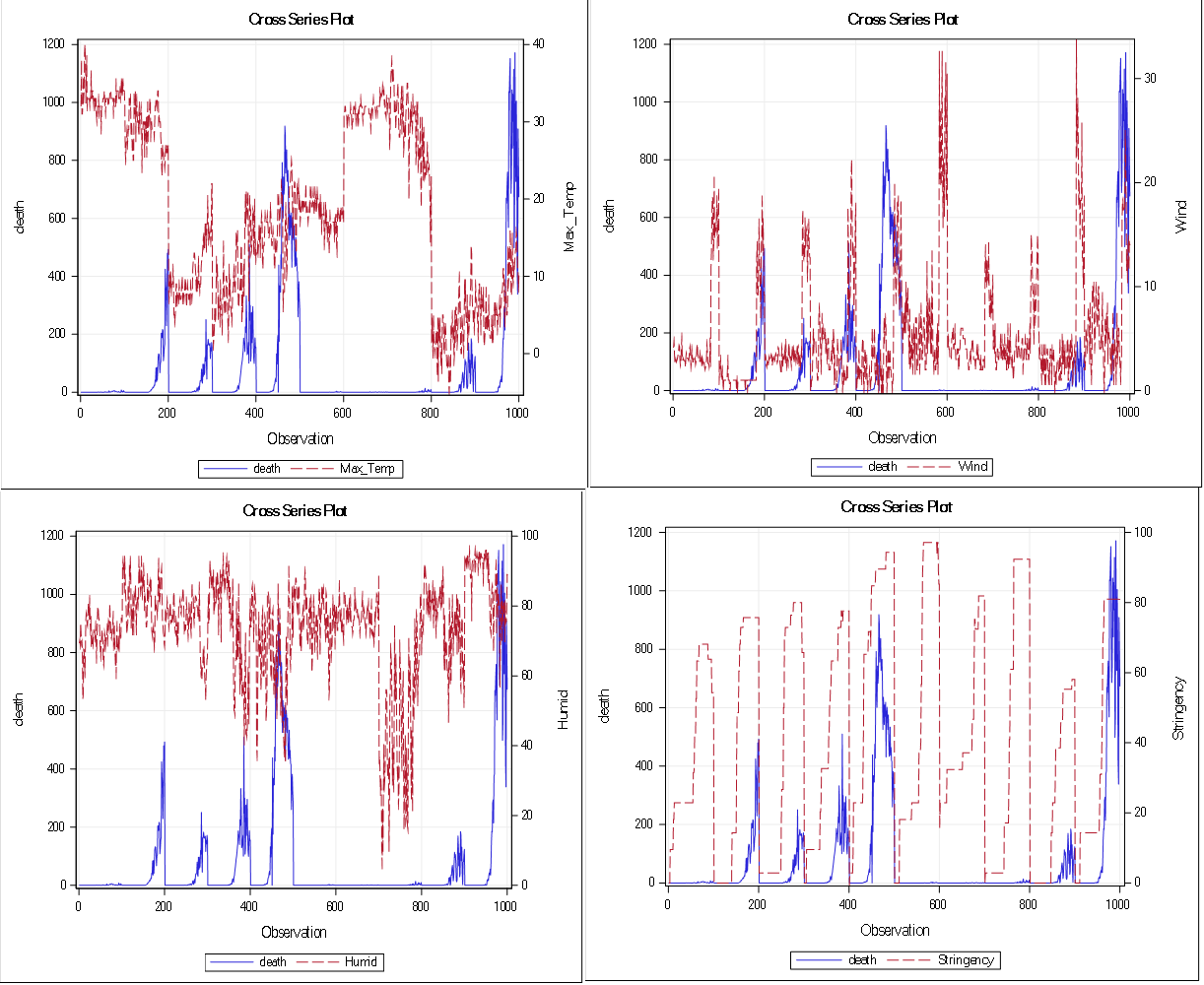
The above correlational analysis also neglects the temporal spatial nature of the data and the order in which they occur. Time is an important aspect of the data generation process. Assuming a 14 days lag, we explore the autocorrelation as well as cointegration of the spatio-temporal relationship amongst these variables. In order to demonstrate this, we generate series plot of dynamic relationship between each of the COVID-19 outcome data (see Figure 2).
One would expect these variables to be highly correlated and this is shown in Figure 2. The dynamics in time are closely related, which confirm the correlation results; recovery and confirmed cases 0.59 (0.54, 0.63) P<.0001, recovery and death cases 0.50 (0.46, 0.55) P<.0001, and confirm and death case 0.84 (0.83, 0.86) P<.0001. However, this type of close association over time, seen in these variables, are not reflected with weather parameters, except stringency index and wind speed (see Figure 3).

According to Figure 3, stringency and death rates are strongly associated over time. Correlation estimates for stringency is 0.69 (0.66, 0.72) P<.0001. Also, death rates are also strongly associated with wind speed (top right of Figure 3), however, the correlation estimate calculated from Spearman’s correlation analysis is 0.18 (0.12, 0.24) P<.0001. Without a visual graphical inspection of these two variables, such an association would not have been captured (as Spearman’s correlation of 0.18 is weak), thus warrants a further analysis.
On the other hand, Figure 4 presents the cross series of recovery rates and the weather parameters. Similarly, it is evident that stringency and wind speed are associated with recovery rate over time with correlation estimates, 0.60 (0.56, 0.64) P<.0001 and 0.22 (0.16, 0.28) P<.0001 respectively.

We generate similar plots for the confirmed cases, see Figure 5. Confirmed cases are positively associated with wind speed and stringency index over time, 0.18 (0.12, 0.24) P<.0001 and 0.80 (0.78, 0.82) P<.0001, respectively.

The autocorrelation for the associations of most of the weather parameters, except wind speed, with COVID-19 outcomes are random, which is ascertained by the near zero autocorrelations.
Finally, we explore relationship and causality, if any, among all the considered variables via a vector autoregressive analysis. Two groups of the variables were created, group one with recovery rates, confirmed cases and death, and group two with maximum temperature, humidity, wind speed and stringency index. The null hypothesis of the Granger causality test22 is that group 1 is influenced only by itself, and not by group 2 and a p-value below 0.05 confirms the dependence.
The findings suggest that there is no evidence of dependencies among the variables with a p-value of 0.1593, which is greater than 0.05. The following relationships were established with coefficients being those with p-values below 0.10.
\begin{align} \mathbf{Recovery\ (t)}\ =& \ 0.70*recovery(t - 1)\ \hspace{32mm}(1)\\ &+ \ 0.27*confirm(t - 2)\\ \\ \mathbf{Confirm\ (t)}\ =& \ 1366.07\ + \ 0.68*confirm(t - 1)\ – \hspace{12mm}(2)\\ &\ 22.26*stringency\left( t - 2 \right)\\ \\ \mathbf{\text{Death}}\left( \mathbf{t} \right) =& \ death\left( t - 1 \right) + \ 2.64*stringency\left( t - 1 \right) \hspace{5mm}(3)\\\ &+ \ 0.22*death\left( t - 2 \right)\ –\\ &\ 2.84*stringency\left( t - 2 \right) \end{align}
The above suggests that recovery at the current time is driven by recovery at the immediate time past and confirmed cases 2 days earlier. Also, confirmed cases at the current time is dependent on an average reported confirmed cases, plus a percentage of the immediate past confirmed cases, less a multiplicative factor of the stringency in the past two days. This seems to confirm what has been found in an unrelated work, suggesting the lock-down date only delay by 3 days, the estimated confirmed cases.23 Similarly, the death reported at the current time is related to the death reported during the immediate time past, a multiplicative of death reported at the immediate time past and a multiplicative of the stringency of the past two days. These results show that confirmed, recovery and death rates do not significantly depend on any of the weather parameters we considered in the research.
Discussion
The arrival of warm weather raised the expectation that the spread of the disease will slow down and the “notorious” curve will flatten. But is it likely? Most studies in the literature noted that temperature and high levels of humidity are associated with lower negative COVID-19 incidences. However, there are serious limitations around the methodological assumptions and the data used in these studies, as explained in the introduction, thus the results can be deemed to be inaccurate and inconclusive. We therefore carried out an exhaustive analysis of data tackling some of these issues for 10 countries from all over the world by considering all continents but Antarctica. Daily confirmed cases, number of deaths, number of recovered cases, lockdown stringency index, several meteorological factors along with other variables (number of hospital beds per 1000 population, hospital occupancy rate, GDP per capita and population density) were investigated in greater detail.
According to the graphical illustrations, there is a clear corelated pattern, between meteorological parameters and COVID-19 pandemic. Explanatory analysis of statistical results tells a different story. The findings suggest that most of the associations reported in the literature need to be interpreted with caution, as most of these articles neglected the temporal spatial nature of the data.
Based on our findings, most of the correlations no matter which coefficient is used are mostly and strictly between -0.5 and 0.5, which are weak correlations. Most of these articles reported p-values but without confidence intervals and without explaining hypotheses that have been tested. Using the Pearson correlation coefficient for our ten-country data, the data suggests weak correlation after we partial out stringency index and minimum temperature.
The Pearson correlation estimates between COVID-19 outcomes and meteorological factors suggest very weak association, ranging from -0.26 to 0.28, with wind being showing the strongest association, albeit very weak.
The correlation estimates show that stringency and death rates are strongly associated over time and similarly stringency and wind speed are associated with recovery rate. Although the correlation estimates are weak in some variables (e.g. death rates vs. wind speed), a visual inspection of the plots reveals a strong association between the variables. The strong correlation estimates for stringency index and COVID-19 outcomes could be explained as, the more cases are confirmed, government put stricter restrictions on movement of people. Also, the more confirmed cases, the more death and recovery outcomes. It suggests that confirmed outcome is a confounding factor between stringency and each of recovery and death outcome.
An interesting but not surprising finding is the correlation between stringency and each of the COVID-19 outcomes, the strongest being between stringency and confirmed cases, 0.80 (0.78, 0.82) P<.0001. However, a negative correlation would be expected between stringency and COVID-19 outcomes, as the higher SI index means a tighter lockdown. Note that countries generally increase the control (SI) as the COVID-19 cases increase. The increase in the figures generally continues for a long period of time (weeks), as a result positive correlation may arise from this trend. Lockdown policies are generally for controlling the increase in the cases. When time passes with lockdown, the figures gradually go down.
Note that there are significant variations on the national differences in COVID-19 diagnosis and reporting of outcomes (e.g. death, recovery, confirmed cases). For instance, the UK reports death in hospital and the community separately causing delay in the number of daily deaths. Also, the number of recovered patients is not available in the UK or it is reported in batches as oppose to daily in Brazil. We attempted to capture the lag and lack of the data in the reporting within our model.
Lastly, a vector autoregressive analysis is carried out to explore any relationship and causality among the variables. The analysis revealed that recovery and death rates do not significantly depend on any of the weather parameters considered in the study. In brief, the studies in the literature mainly lack evidence and clear interpretation of the statistical output (e.g. underlying assumption, confidence intervals, a clear hypothesis). To uncover the devil hidden in the detail, a comprehensive and exhaustive analysis along with proper interpretation of graphical outputs and statistical analysis are essential. Based on this explorative analyses, statistical results in many articles reporting association between meteorological parameters and COVID-19 outcomes need to be interpreted with caution, especially when the spatial-temporal nature of the data generation process is ignored, the devil might be in the details.
Future works
As an extension of this study, we will jointly model longitudinal meteorological factors with COVID-19 outcomes, adjusted for key covariates, such as GDP per capita, number of intensive care unit (ICU) beds, deprivation score and stringency index. Thus, it is expected that (1) the trajectory over time (evolution) of COVID-19 incidence will be related to the evolution of a meteorological factor, as one may have direct and indirect implications on the other, and (2) the effect of covariates may not be captured if we ignore the interdependence in the evolution of these outcomes. The advantages of the joint modelling approach are the ability of accounting for interdependence by bringing together the models for each outcome (both COVID-19 incidences and meteorological factor) by specifying a joint distribution for their random effect terms.
Conclusion
Our exhaustive analysis showed that the associations reported in the literature need to be interpreted with caution, especially when the spatial-temporal nature of the data generation process is ignored, the devil might be in the details. A notable shortcoming of this study is the period for which the data have been collected and the variability in the countries considered, especially in the position along the course of the pandemic. The authors think that, time will tell if really there are any strong associations between meteorological parameters and the pandemic. However, without effective control measures, strong outbreaks are likely in more windy climates and summer weather, humidity or warmer temperature will not substantially limit pandemic growth. Therefore, we postulate that the drivers would be more related to the way of life, urban population density, healthcare system preparedness and socio-economics characteristics.
Funding: None
Authorship contributions:
All authors have contributed to the study equally. The manuscript has been reviewed, edited, and approved by all authors.
Competing interests:
The authors completed the Unified Competing Interest form at www.icmje.org/coi_disclosure.pdf (available upon request from the corresponding author), and declare no conflicts of interest.
Correspondence to:
Usame Yakutcan
PhD, AFHEA, MSc, BSc
Hertfordshire Business School
University of Hertfordshire
Hatfield, UK
[email protected]