


The objective of the current work was to develop a simple predictive model of the spread of novel coronavirus (i.e., 2019-nCoV or SARS-CoV-2) in the United States. In the US, the response to the pandemic varies greatly from state to state. As state government policymakers evaluate different mitigation and containment measures, they rely on various models to predict the trajectory of the outbreak in response to their proposed policies. The purpose of the work is to develop a simple, fast running model that could be easily applied to understand the consequences of different policy decisions on a state-by-state basis. Ideally the model would be easily understood, both to use and interpret the results, by people without expertise in epidemiology. The model developed is based on the SIR concept and coded in Python with a simple text-based input. The code incorporates strategies for mitigation and containment and can be adjusted for application to various states with changes to only a handful of key input parameters.
Methods
The current SEIR+AQ model builds on the work of Tang, et al.1,2 The basic principle is to divide a given population into subpopulations and establish a series of differential equations that describe the changes in those subpopulations. The SEIR+AQ model is comprised by equations that dictate the change in each of the subpopulations (e.g, susceptible, exposed, etc.) but ancillary equations are added to compute different figures of merit. The figures or merit for the SEIR+AQ model include the number of people testing positive for COVID-19, the number of people hospitalized and the degree of care they need, and the number of virus-caused fatalities. The SEIR+AQ subpopulation results are used as inputs to the ancillary equations to drive these equations and predict the number of cases, casualties and hospital resource utilization.
In addition, the equation parameters can be manipulated at discrete points in time to implement or revoke mitigation or containment strategies. Four strategies are considered in the model: (i) social distancing, (ii) mask wearing, (iii) temperature monitoring, screening, and quarantining, and (iv) contact tracing and quarantining.
SEIR+AQ subpopulation continuity equations
The population being analyzed (i.e., a state or city) is initialized with a given population size, typically the most accurate population estimate. Within that population, there is assumed to be a single infected individual (I(0) = 1) and the remainder of the population make up the initial susceptible subpopulation (S(0) = population – 1). Initially, all other subpopulations are not populated (i.e., E(0)=R(0)=A(0)=Q(0)=0). From this point, the rates of change in the subpopulation are computed according to the following system of equations. These rates of change are used to compute changes in the population over discrete time steps. In the current SEIR+AQ model, the time step is set to one hour.
The susceptible population rate of change decreases as people become infected with the virus. The susceptible population may be infected due to contact and transmission with infectious individuals in the wider population or by infection from individuals in the quarantined population. The model recognizes that the wider population has a more frequent rate of contact than individuals that are quarantined. This is represented in Equation 1.
S′= −β c S (ζE+I+A)− βS(ζEq+Iq)(1)
Where S’ is the rate of change of the susceptible population,
β is the transmission probability per contact,
c is the contact rate,
S is the susceptible population,
ζ is the relative infectiousness of an exposed vs. an infected individual,
E is the exposed population that is not under quarantine,
I is the infected population that is not under quarantine,
A is the asymptomatic carrier population,
Eq is the population of exposed individuals that are quarantined, and
Iq is the population of infected individuals that are quarantined
A new feature included in Equation 1 that is absent from Tang’s model is the inclusion of an infection pathway where pre-symptomatic, exposed individuals have some chance to spread the infection. A factor (ζ) dictates the relative transmission probability of a pre-symptomatic, exposed individual relative to a post-symptomatic (i.e., infected) individual. This factor was added because research suggests that pre-symptomatic individuals can spread COVID-19.3,4
Equation 2 shows the equation for the exposed population. The source term for exposed individuals is given by the transition of susceptible persons that are exposed to the virus. An implicit assumption of the SEIR model is that individuals who recover from COVID-19 are immune to reinfection, so there is no source term in Equation 2 representing possible reinfection.
There are two sink terms. The first is given by the rate at which exposed individuals develop symptoms and are transitioned to either the infected or asymptomatic carrier classes. The second sink term is associated with potential containment strategies. The containment strategies are discussed in greater depth below. For now, this second sink term dictates the rate at which exposed individuals are placed under quarantine through contact tracing.
E′= β c S (ζE+I+A)+ βS(ζEq+Iq)−σE−c(TMF)(TMS)(TMC)FDPI[(CTF)(CTE)ES+E+I+A](2)
Where E’ is the rate of change in the exposed population,
σ transition rate from exposed to infected (i.e., one divided by the incubation time)
TMF is the temperature monitoring flag, it has a value of 1 if temperature monitoring, screening and quarantine measures are in place,
TMS is the temperature monitoring/screening fraction – it is the fraction of the unquarantined population that is subject to temperature measurements as part of routine screening,
TMC is the compliance fraction – it is the fraction of individuals who have high temperatures (i.e., showing COVID-19 symptoms) that will comply with the order to quarantine,
FDP is the number of days following the appearance of the first COVID-19 symptoms before an individual has a measurable and actionable fever. What it means to be “actionable” is further described later in this paper.
CTF is the contact tracing flag – it has a value of 1 if contact tracing measures are in place, and
CTE is the contact tracing effectiveness – it is the fraction of contacts between an individual entering quarantine and a member of the public that has been exposed that the contact tracers can identify.
Exposed individuals that are in quarantine are tracked in the SEIR+AQ model. The source term in Equation 3 comes from individuals placed under quarantine through contact tracing and the sink term is the rate at which the virus incubates to full infection and the exposed individuals transition to the infected (but still under quarantine) class.
E′q=c(TMF)(TMS)(TMC)FDPI[(CTF)(CTE)ES+E+I+A]−σEq(3)
The at-large infected population rate of change is given by Equation (4).
I′= σρE−αI−γI−(TMF)(TMS)(TMC)FDPI(4)
Where ρ is the fraction of infections that lead to symptoms,
α is the death rate, and
γ is the recovery rate.
Analogous to the exposed, quarantined population rate of change shown in Equation 3, an equation is developed for infected persons under quarantine, see Equation 5. Here there are two source terms: (i) individuals that are quarantined as a result of temperature monitoring and screening and (ii) those that were quarantined from contact tracing but developed symptoms later. The sink terms are given by the rates of death and recovery.
I′q=(TMF)(TMS)(TMC)FDPI+σEq−αIq−γIq(5)
The total quarantined population (Q) is found simply by summing Iq and Eq.
The asymptomatic carrier subpopulation (A) is calculated by Equation 6. It is noteworthy that asymptomatic carriers, as they do not express symptoms, do not have any identified increase in hospitalization or fatality rates. Therefore, Equation 6 does not have a sink term associated with virus-induced death.
A′= σ(1−ρ)E−γA(6)
The removed subpopulation (R) includes those that recover from the disease (and are therefore no longer susceptible) as well as those that die from the disease. It is calculated according to Equation 7.
R′=(α+γ)(I+Iq)+γA(7)
The removed subpopulation includes both recovered and decreased individuals. For computing different figures of merit, the recovered subpopulation components or recovered individuals and casualties are also tracked.
These equations form the SEIR+AQ model and are solved numerically by taking discrete time steps, computing the rates of change, and updating the respective populations by summing them with the product of the rate of change and the time step.
Calculation of cases
For validation of the model, the predictions must be compared to available data. In the current work, the number of cases is used as a figure of merit. An ancillary set of equations has been added to calculate the resultant number of cumulative cases. The current approach assumes that infected people with severe symptoms will be administered a diagnostic test. The positive tests are then tallied cumulatively to produce the number of cases.
The model does not consider non-infected individuals with COVID-19-like symptoms getting tests. While this occurs in the population, and there will be some false positive results from those tests, the contribution to the case number does not significantly contribute to the error relative to the other uncertainties and can be ignored.
Additionally, the model presumes that cases are reported only for those individuals that receive a positive diagnostic test result. Early in the infection outbreak, testing was not widely available in the US, and therefore, many cases were identified based on presumptive diagnosis on the basis of the symptoms expressed. The fraction of these presumptive cases should decrease with time as testing becomes more widely available in the US. Therefore, the model should produce a strong bias in underpredicting the cases early in the simulation, but the bias should decrease as the rate of testing and number of cases increases.
The testing rate is calculated according to Equation 8. The rate at which infected persons are tested is first computed by taking the rate at which people become infected. This rate is then multiplied by a factor (χ). This factor represents a screening of testing eligibility. Lastly there is a time delay to account for the period between a test being administered and the result.
T′=χσρ(E(t−ψ)+Eq(t−ψ))(8)
Where T’ is the rate at which infected individuals test results accrue,
χ is the fraction of infected individuals with symptoms that express symptoms severe enough to warrant diagnostic testing, and
ψ is the number of days from receiving a diagnostic test before the result is known.
The number of identified cases at any point is time is computed by taking the number of tests performed on COVID-19 patients and reducing this by a factor to account for false negative results. The cumulative case number is calculated as shown in Equation 9.
C=(1−ε)T(9)
Where C is the cumulative number of cases and,
ε is the false negative probability for the test.
Calculation of hospital resources needed
The hospitalization rate is calculated similarly to the SEIAR+AQ subpopulation calculations. The source term for the hospitalized subpopulation is related to the rate of new infections, as individuals transition from the exposed to infected class, after some period once symptoms manifest, those symptoms may become sufficiently severe that hospitalization is warranted or required. Individuals leave the hospitalized population by: (i) developing worsening symptoms that requires intensive care, (ii) recovering sufficiently to be discharged, or (iii) dying. Equation 10 shows how the hospitalization rate is computed.
H′=κσρ(E(t−λ)+Eq(t−λ))(10)−(μν+3γ+α)H
Where κ is the probability that an infected individual’s symptoms will be so severe as to warrant hospitalization,
λ is the time from the onset of symptoms until they worsen to the point where they are sufficiently severe to require hospitalization,
μ is the probability that once hospitalized, the patient’s symptoms continue to worsen to the point where intensive care is required, and
ν is the rate at which patients are transferred from conventional hospital treatment to intensive care.
Three items of note in Equation 10 are worth clarification. First, the equation utilizes the exposed population because this dictates the rate of new infections and the hospitalization rate depends on how many people developed symptoms λ days in the past.
Second, patients whose symptoms worsen to the extent that intensive care is required are subtracted from the hospitalized subpopulation and are added to the intensive care subpopulation. There is a sink term in the so-called hospitalized subpopulation for patients transferred to intensive care, but that patient is still technically hospitalized. Therefore, when using these results to determine the peak resources required, the hospitalized subpopulation result must be summed with the intensive care and intubated subpopulations to give a picture of the total number of people in the hospitals.
Third, the recovery rate in Equation 10 is tripled. This does not affect the rate of recovery in the at-large population and does not affect the progression of the infection in the underlying population. Rather, this factor reflects that patients will be discharged from the hospital once they are partially recovered but not fully recovered.
Patients that are hospitalized but develop worsening symptoms will be transitioned to intensive care. The rate of change of the intensive care population is shown in Equation 11. The source term comes from the transition or hospitalized patients and the sink term has three components: death, recovery, or the possibility that symptoms worsen further still and require intubation.
ICU′=μνH−(οτ+γ+α)ICU(11)
Where ICU’ is the rate of change of the intensive care population (not intubated), and
ο represents the conditional probability that a hospitalized patient in intensive care will develop worsening symptoms requiring or warranting intubation, and
τ is the rate at which patients transition from intensive care to requiring ventilators
As with the hospitalization rate, the intensive care rate does not consider patients on ventilators to be part of the intensive care unit. The ICU population must be summed with the population on ventilators (V) to represent the total number of patients in intensive care (both intubated and not). The last piece then is to account for the ventilator population, which is shown in Equation 12.
V′=(οτ)ICU−(α+γ)V(12)
Where V is the rate of change in the number of patients on ventilators.
Given this system of equations, the results from the SEIR+AQ model can be used as a driver to calculate the hospitalized, intensive care, and intubated populations.
Modeling mitigation and containment strategies
This section describes how various mitigation and containment strategies are modeled. It should be noted that because this model was developed primarily for application to the US, it does not consider containment strategies that rely on widespread testing access. The following sections describe the specific mitigation and containment strategies currently modeled.
Social distancing
The model allows a social distancing order to be imposed. The effect of the order is to change the normal contact rate to a lower contact rate. In the work by Tang, et al., the contact rate would decrease over time from an initial value to a value consistent with the present mitigation orders. While an order can be imposed in one day and enforced the next in the US – which motivated the use of step function change in the contact rate – many states in the US issued a variety of social distancing policies over the course of several days. For example, in Washington, DC, there was an order to close schools, then some days later, an order to close non-essential businesses, and then some days later a stay-at-home order. While each individual order went into effect on a given day, the various orders had the effect of ramping up the social distancing effect over several days. So, while in the development of the SEIR+AQ model, the approach of Tang, et al., was eschewed, Tang, et al.'s method is probably more accurate. Regardless, reasonable agreement could be found with state-by-state validation data if a single social distancing order was imposed in the model, representing a date between the first and last of the piece-wise social distancing policy enactments.
To use Washington, DC as an example to illustrate the social distancing order model, the first case of COVID-19 was identified on March 7, 2020. On March 16, schools were closed; on March 25, non-essential businesses were closed; and on March 30 the mayor issued a stay-at-home order. To determine the day that would represent the social distancing order in the model, the average of the non-essential business closure and stay-at-home order (30-7+25-7)/2 was used, which gives 20.5 days. This was rounded down to 20 days because the school closure took place earlier.
In the model, 20 days after the first case is identified (when C increases above one), the contact rate (c) changes from the normal rate to a socially-distant-contact rate, which is smaller.
Mask wearing
The model can account for mask wearing. The model simulates a mask wearing order by adjusting the transmission probability per contact (β) by applying a reduction factor (M). The transmission reduction factor accounts for several characterizing factors, including the effectiveness of masks as well as the fraction of the population wearing masks. As for the former, the effectiveness of a mask in reducing the transmission for an individual was assumed to be 60 percent. In the actual population a variety of face coverings will be used. Essential medical workers may be using highly effective N95 masks while others may be using surgical masks or home-made masks, or even simpler face coverings. Therefore, this parameter (average mask effectiveness) is largely conjectural. An April 2020 news article5 provided a comparison of different face coverings in terms of their filtration ability relative to airborne particles and provides 60 percent as the lower end of the range for surgical masks relative to small particles (< 0.3 μm). The World Health Organization (WHO) described the primary transmission mechanism as being through respiratory droplets (> 5 μm) or through direct contact.6 On this basis, a 60 percent effectiveness of masks was used in the model as it appears to represent the lower end of the medical-grade protective equipment range and at the same time the upper end of the hand-made mask range.
Given the mask effectiveness, the overall impact on the transmission probability must consider the effect on both a potential infector and a susceptible person in a contact. In our model we assume that all essential workers will wear masks and that some fraction of non-essential workers will don masks. The fraction of non-essential workers that wear face masks is a cultural parameter and will vary between populations. As a default, the model uses a 50 percent value, but this value can be updated to reflect a specific population. The transmission probability reduction factor can be calculated now according to Equation 13.
M=[(e+(1−e)f)(1−m)+(1−e−(1−e)f)(1)]2(13)
Where M is the mask-wearing transmission probability reduction factor,
e is the fraction of the population considered to be an essential worker,
f is the fraction of non-essential workers that voluntarily don face coverings, and
m is the effectiveness of a mask (on-average) to reduce transmission.
In the model when mask-wearing is imposed, the transmission probability per contact (β) is multiplied by the reduction factor (M).
It should be noted that this model of the mask reduction factor assumes that the mask-wearing confers not only a benefit in that it reduces the transmission from an infected person, but also that a mask reduces the likelihood that a susceptible person who has contact with an infected person will contract SARS-CoV-2. While the efficacy of masks to reduce onward transmission from an infected person has been established,7 the model assumes a benefit also to a susceptible person wearing the mask – this is a conjectural feature of the model at the current time and may not be accurate.
Temperature monitoring, screening and quarantine
The temperature monitoring, screening and quarantine containment strategy is based on using work-place based temperature measurements to screen workers and determine who has a fever. People with a fever are then directed to self-quarantine until they have recovered. The model simulates this by adding another subpopulation (Iq) which tracks those that are infected but have been quarantined. It should be noted here that there will be many individuals in the population who show signs of a fever, but do not have COVID-19. The model right now does not consider the impact of quarantining susceptible individuals with non-COVID-19, fever-inducing illnesses. This is a conservatism in the modeling that will under-estimate the efficacy of the quarantine because the susceptible individuals are still modeled as having a normal contact rate.
Equation 4 and 5 show how quarantining based on temperature monitoring and screening is modeled. There is a sink term in the infected population equation that appears as a source term in the infected-quarantined population equation. This term has several factors: TMF, TMC, TMS, and FDP.
TMF is the temperature monitoring flag – this flag is set to unity when there is an active temperature monitoring order in the model.
TMC is the temperature monitoring compliance fraction. This is a cultural parameter and represents the fraction of individuals who are ordered to quarantine that will abide by the order to quarantine. This parameter can be controlled by user input, but the value will be set to the fraction of people wearing masks by default. This is computed by the Equation 14.
TMC=e+(1−e)f(14)
TMS is the temperature monitoring screening. This is another cultural parameter and represents the fraction of individuals who are subject to have their temperatures regularly taken as part of the containment strategy. Because the strategy envisions that people will be monitored at their places of work, the TMS should reflect the fraction of the population that are working for an employer at a fixed place of business.
FDP is the fever development period. This is a virus-specific model parameter and it represents the time after the onset of symptoms before an infected person will have a measurable fever.
The current model assumes that all symptomatic individuals will express a fever. This is based on the research of Wang, et al., who have shown fever to be the most common symptom among patients in Wuhan and to be a nearly universal symptom of the infection (much more universally prevalent as a symptom than any other symptom).8 However, if it is later shown that fever is a less common symptom among the symptomatic population, then this could be accounted for by reducing the TMS factor.
Contact tracing and quarantine
The temperature monitoring, screening and quarantining containment strategy might be augmented with a contact tracing program. Contact tracing relies on doing research to establish individuals that have had contact with a suspected infected person. In the model this is implemented by quarantining exposed individuals that have had contact with an infected person that has been ordered to quarantine. For simplicity in developing the numerical solution, it is assumed that the quarantine compliance fraction is the same for infected or exposed individuals. This has the effect in Equations 2 and 3 of removing at-large exposed individuals to quarantine at a rate proportional to the rate at which infected individuals enter quarantine.
There are additional factors in the subpopulation equations: (i) CTF, (ii) CTE, and (iii) cE/(S+E+I+A). The CTF is the contact tracing flag, it is set to 1 if contact tracing is active in the simulation.
When contact tracing is active, the model will calculate the rate of infected people entering quarantine according to the temperature monitoring, screening and quarantine model. The contact tracing model assumes that each of these infected quarantined individuals will lead to the identification of some number of exposed individuals in the at large population, and those exposed individuals will also move into quarantine. Since the compliance is assumed to be the same, this means that this can be thought of as all exposures from a complaint infected quarantined person as also complying with quarantine. An infected person may not abide by a quarantine order, but the contact tracers may identify an exposure that would lead to self-quarantine and the inverse may also occur.
Contact tracing has an effectiveness (CTE) that characterizes how effective the contact tracing program is in identifying a person’s contacts that led to exposures. This effectiveness is multiplied by the total number of contacts (c) and the likelihood of the contact having led to exposure (which is computed as the ratio of the exposed-at-large population to the total-at-large-population). The CTE is a cultural parameter that will vary based on population. Since large scale contact tracing programs have not yet been demonstrated in the US, selection of any value for the CTE is conjectural. Currently the model uses a default value of 0.25.
This product gives the rate at which contact tracing identifies exposed individuals and moves them into quarantine. Once in quarantine, an exposed individual is assumed to remain in quarantine as they progress to an infected status. Therefore, the term σEq appears in Equation 5. Even though some exposed individuals in quarantine will become infected but express no symptoms, this model treats these asymptomatic individuals as remaining in quarantine through the course of their infection.
Parameter values
The model description above relies on the specification of several parameters that characterize the virus and its spread. Online Supplementary Document (OSD) Appendix S1 describes the virus-specific model parameters and OSD Appendix S2 describes the population-dependent or “cultural” parameters.
Concept of infection multiplication
SARS-CoV-2 has been characterized in the literature according to a virus reproduction number (R0) which tells how many secondary infections will stem from a primary infection and this value in the literature is approximately 2.5 (2.4 from9 and 2.5 from10). Many models seem to determine an “effective” or “control” reproduction number to characterize how mitigations change the infection rate. In the current work, a new approach is proposed to use an effective infection multiplication factor to function in a similar capacity.
The effective infection multiplication factor (keff) could be understood in a manner similar to the time dependent reproduction number in that keff characterizes if infections are expected to increase, decrease, or hold constant. It can be calculated by solving the eigenvalue problem for the infected subpopulation continuity equation. By combining Equations 4 and 5 we get an expression for the total infected population – since Equation 5 only deals with the quarantine based containment strategies, the net effect on Equation 4 by combining with Equation 5 is small because one is both adding and removing the quarantine population and then separately tracking exposed individuals in two subpopulations. However, the principle of keff can be explained with just Equation 4 if one ignores quarantine.
If one rewrites Equation 4, ignoring the difference between the at-large and quarantine populations, as a steady-state eigenvalue problem then one arrives at Equation 15. Below Equation (15) is written as the eigenvalue problem and then rewritten again in terms of keff.
0= ΛσρE−(α+γ)I(15.1)
(α+γ)I= σρEkeff(15.2)
Where Λ is the eigenvalue.
From Equation 15 it is clear how to interpret keff. It is a ratio of the sources to sinks in the infected population continuity equation. When keff is greater than one, the infected population is increasing and conversely it is decreasing when keff is less than one. Factors that affect the keff can be shown simply by rearranging Equation 15 as Equation 16.
keff= σρ(α+γ)EI(16)
Factors that increase the rate of new infections (by affecting E) increase keff while factors that promote recovery (by affecting I) decrease keff. It is clear from Equation 16 how applying social distancing would decrease keff as it would cause a decrease in the exposed population before it would affect the infected population. Additionally, one can see immediately how the advent of a novel treatment that could improve the recovery rate would affect the keff. If a treatment were discovered that increased the recovery rate (γ) this would also decrease the keff. Therefore, it has a similar analytical purpose as the reproduction number. In the code the instantaneous keff is calculated according to Equation 16.
When casting the keff in terms of the eigenvalue it can be thought of intuitively as the ratio of the infected population in one generation divided by the infected population in the previous generation of the infection. The generation time is taken as the incubation time. The keff at any time in the simulation can be used to forecast the infected population one generation time later according to Equation 17.
keff(t)=I(t+1/σ)+Iq(t+1/σ)I(t)+Iq(t)(17)
With this intuitive understanding of keff one can see that, as an example, a value of 2.0 would mean that the infected population would double in one generation time (5 days). Correspondingly, if keff is 0.5, the infected population would be reduced by 50 percent in one generation time.
From the definition of the multiplication factor its relationship to the “curve” is apparent. A value greater than one indicates a growing trend in infection and larger values of keff indicate the magnitude of the rate of growth. What this quantification introduces, however, is not only a metric to describe whether the “curve is bending,” but it also allows an analyst to evaluate and quantify the effectiveness of different control measures (i.e., mitigation and containment strategies) and may serve as a useful tool when it comes to deciding on appropriate policies.
Concept of control measure worth
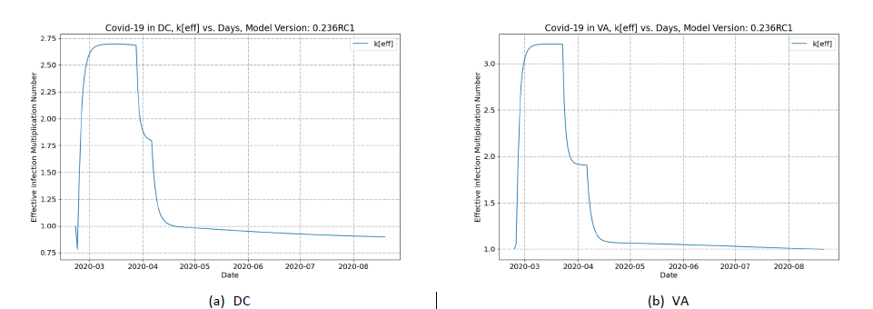
The change in the infection multiplication factor in response to a change in policy can be used to quantify the worth of that policy in combatting the spread of the infection. To further illustrate this concept, it is useful to refer to examples. Therefore, results of the SEIR+AQ model for two examples will be discussed in terms of the changes in keff as different mitigation strategies are employed in two populations. Briefly, the calculations described simulate the SARS-CoV-2 outbreak in the District of Columbia (DC) and Virginia (VA), respectively. The calculations account for two mitigation strategies: social distancing and mask wearing.

Figure 1 panel A shows the evolution of keff over 180 days. The “blip” in the curve on the first day is a numerical artifact of the solution and should be ignored. The keff grows rapidly and stabilizes at the initial value of ~2.7. This initial value is much akin to the concept of the initial reproduction number for the virus (R0). It characterizes the progression of the infection when there are many more susceptible individuals in the population relative to infected individuals.
There is a dramatic decrease in the keff once social distancing orders are put in place (near the end of March), when the keff drops from a value of ~2.7 to a value of ~1.8. After this drop there is another sudden decrease (in early April), this second drop occurs when mask wearing guidance was issued and this results in the keff dropping to a value below one. After these mitigation measures are implemented the keff continues to decrease over time.
The subsequent and continued decrease of keff is indicative of the buildup of herd immunity. The susceptible class can be thought of as providing the fuel that feeds the infection. The slow, steady decrease in keff with time reflects a kind of fuel depletion as the population approaches herd immunity. Herd immunity can be said to be achieved when the keff remains below one even when mitigation and containment measures are lifted as this will indicate when the susceptible individuals in the population are so sparse that the infection’s spread is stifled.
From this discussion one can see how the current model could be used to predict when herd immunity has or will be established. One could use the model to conduct numerical sensitivity analyses where the mitigation or containment strategies are removed and the keff is calculated. When the keff without controls remains below one, herd immunity has been established.
However, this shows that the mitigation measures of imposed social distancing and mask wearing have a substantial effect on the progression of the infection. In this case these measures are predicted to have a sufficient effect that the keff is reduced below one, indicating that the infections should decrease. The relative importance of the two measures can now be quantified in terms of their worth. The difference in the multiplication factor is used to establish how valuable (the worth) of the mitigation measure is in terms of the impact on infection multiplication. This can be computed by taking the difference in the inverse of the multiplication factor before and after the measure is imposed. Using our example for Washington, DC, the worth of the social distancing order can be computed according to Equation 18.
W=[1keff]before−[1keff]after(18)
Where W is the worth of the measure.
For social distancing, the worth is -0.19 and for mask wearing the worth is -0.45. These two control measures are sufficient to control the entire worth of the virus itself (which is 1/1-1/2.7 or 0.63). Since one needs to know the worth of a control measure relative to the worth of the virus itself, the control measure worth is normalized to the virus worth and the result is reported in units of dollars ($) where one dollar corresponds to the same worth as the virus.
Now one can see how control measure worth can be used as a means for constructing a sensible mitigation or containment strategy. The objective of policymakers will be to design a portfolio of mitigation and containment control measures through different policies such that the sum of the worth of the portfolio is -1$. In the example for Washington, DC above, the two measures combined have sufficient negative worth, i.e. -30¢ + -71¢ = -1.01$, which is slightly more (in magnitude) than -1$ and the total portfolio of control measures causes keff to drop below one. If the combined portfolio worth magnitude is less than 1$, then there is not enough negative worth to overcome the virus and the keff would remain above one.
Having demonstrated the concept of worth on the Washington, DC example, it is worthwhile to consider the effect of mitigation and depletion in a second example (VA). The keff results for the VA simulation are shown in Figure 1 panel B. The trend in keff for VA is very similar to the result for Washington, DC. The initial keff is slightly higher, ~3.2. There is a decrease in response to social distancing, to ~1.9, and a second decrease in response to mask wearing, ~1.1. Using Equation 18 the respective worth of the social distancing, and mask wearing can be calculated as -30¢ and -55¢, respectively. Combining the mitigation strategy worth yields a combined worth of -85¢, which (in magnitude) is less than ‑1$. Therefore, the keff remains above one and the calculation predicts that these measures are not sufficient to suppress the outbreak. Consequently cases, casualties, and hospitalizations continue to grow. These will grow until the effect of depletion is sufficient to compensate for the remaining worth (15¢ shortfall after accounting for the -85¢ from the control measures) to squelch the growth in August.

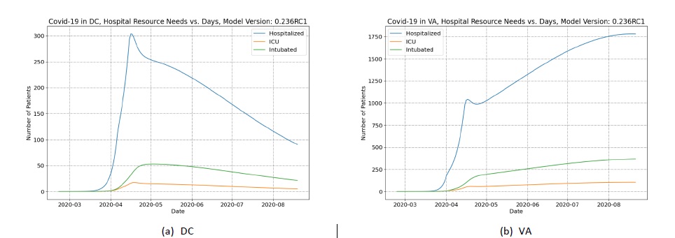
To illustrate the stark difference in consequences, Figure 2 panel A shows the projected hospital resource needs in Washington, DC while Figure 2 panel B shows the projected hospital resources needs in VA. For this comparison it is more important to observe the differences in the trends in the hospital resource utilization rather than the absolute magnitude of the resource needs. The hospital resource needs in Washington, DC peak, plateau and then decrease during the simulation period whereas the hospital resource needs initially peak in VA in mid-May but rather than plateauing, they experience a brief decline before they continue to increase until August. The second peak in August in VA is more than 750 additional beds needed compared to the first peak.
This 15¢ shortfall of the mitigation portfolio in VA illustrates how the missing worth must be compensated by a buildup of recovered individuals in the population. Since the depletion process is slow, compensating even a small budget shortfall in the portfolio can mean many more infections, hospitalizations, and casualties.
Verification and validation
The SEIR+AQ model was verified by comparison to the IHME model and shown to have reasonable agreement (see OSD Appendix S3). In addition, the SEIR+AQ model has been validated against data from several states in terms of the cases and casualties as shown in OSD Appendix S4. The validation shows reasonable agreement with the available data.
Results
A containment strategy for the District of Columbia
The SEIR+AQ model was used to predict the consequences of reopening Washington, DC (i.e., revoking social distancing orders so that the contact rate returns to normal) on May 6, 2020. Mask wearing guidelines remain in place in all calculations. Three scenarios were considered in the analysis to demonstrate the cumulative worth of the policies. In the first scenario, the social distancing orders are revoked without any containment strategy. In the second scenario, social distancing orders are revoked, but a temperature monitoring-based containment strategy is in place. In the third scenario, the containment strategy is augmented with contact tracing and quarantining individuals who had contact with a person showing a fever. The reopening without containment scenario (the first scenario) is analyzed to examine the relative worth of the containment strategies in the second and third scenarios.
Figure 3 panel A shows how hospital resources needs change following a postulated reopening scenario without containment. These resource predictions can be compared to the results shown in Figure 2 panel A (which simulates continuous social distancing orders). The previous peak of ~300 is dwarfed by a new peak of > 1,700 in July.
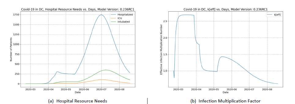
Figure 3 panel B shows the infection multiplication factor in the reopening without containment scenario. Revoking the social distancing order results in the keff increasing from 0.97 to 1.43 which corresponds to a worth of 52¢. Given this worth of the social distancing order, containment strategies can be studied to determine if the containment is sufficient to overcome this positive worth.
The first containment strategy modeled is to impose temperature monitoring, screening and quarantining on the same day the social distancing order is revoked (i.e., on May 6). The results of the temperature monitoring-based containment scenario are shown in Figure 4 panel A. The effect of the policy in terms of hospital resources can be seen in the peak resource usage in July. Without containment of any kind the peak hospitalization was > 1,700 and in the second scenario this is reduced to < 500.
The multiplication factor was used to see the net worth of the combination of the relaxation of social distancing with the temperature monitoring, screening and quarantining. The net effect is an increase in keff to 1.22 indicating a total worth of 33¢. Meaning that the temperature monitoring, screening and quarantining policy has a worth of 19¢. The shortfall of 33¢ would be compensated by susceptible population depletion – and this is reflected in the increase in infections as a result of the policy change.
Consequences could be even further reduced if the worth of the containment policy is increased to reduce the spread of the infection after social distancing is relaxed. Therefore, a third scenario was simulated where the temperature monitoring, screening and quarantining policy is augmented with a contact tracing and quarantining program.
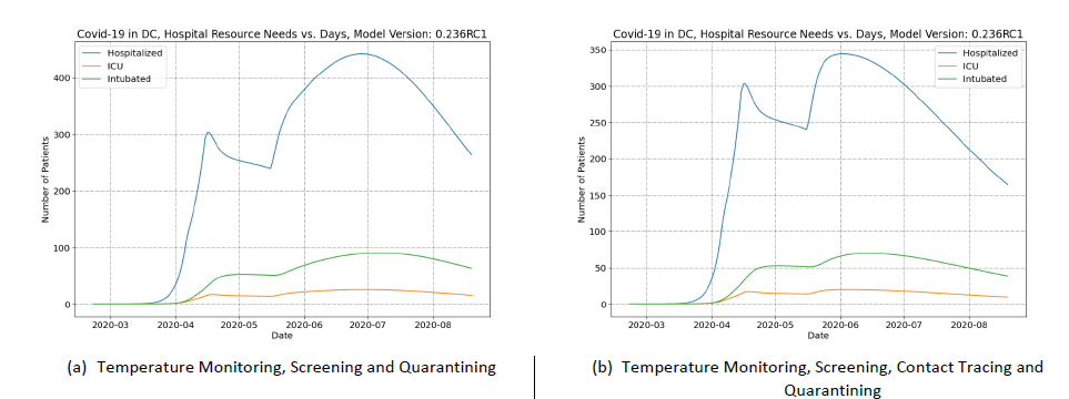
In the third scenario, the hospital resource needs are even further reduced. Peak hospital resources are only slightly greater than the peak in April and it occurs in June (as opposed to July in the previous scenario). Figure 4 panel B shows the hospital resource needs in the third scenario. The contact tracing measure increases the overall worth of the containment policy, but only be a small amount. The net worth of the combined policy is 21¢ compared to temperature monitoring, screening and quarantining alone, 19¢, but even this small increase has a significant benefit in terms of the hospital resource needs.
These scenario simulations show the significant benefits of containment strategies when states attempt to reopen their economies. In addition, the example for Washington, DC illustrates how the concept of infection multiplication and policy worth can be used to evaluate portfolios of different control measure policy options when reopening and which of those policies are likely to confer the greatest benefits to reducing hospital resource needs to acceptable levels.
In terms of casualties, there are consequences to relaxing social distancing policies. In these examples, the containment policy portfolios never contained enough negative worth to overcome the positive worth introduced by revoking social distancing. As a result, the shortfall is made up by an increase in infections. Table 1 compares the total casualties predicted over a 6-month period for the three reopening scenarios and compares them to a base case where social distancing orders remain in place. The results show that reopening early does have a grim cost in terms of fatalities, but it also shows how employing containment strategies and augmenting those containment strategies can reduce the consequences to reopening.
Consequences of relaxing social distancing in Georgia
Georgia was one of the first states in the US to relax social distancing and begin to reopen large sectors of their economy. Two calculations were compared, one where social distancing measures remain in place indefinitely and another where social distancing orders are fully revoked on April 24 and the contact rate returns to the normal contact rate. In the reopening scenario, no containment strategies are simulated.
Figure 5 shows the reference prediction result where social distancing remains in place through the entire simulation. These results are compared to the prediction of a sudden reopening with no containment strategy (shown in Figure 6).

The second peak in Figure 6 panel A vastly exceeds the first peak experienced in April and also greatly exceeds the hospital capacity of GA (~8,200 beds according to5). The hospitalization grows at a tremendous rate in this calculation because the model indicates that the infection multiplication number does not drop below one before the simulated reopening (see Figure 6 panel B).
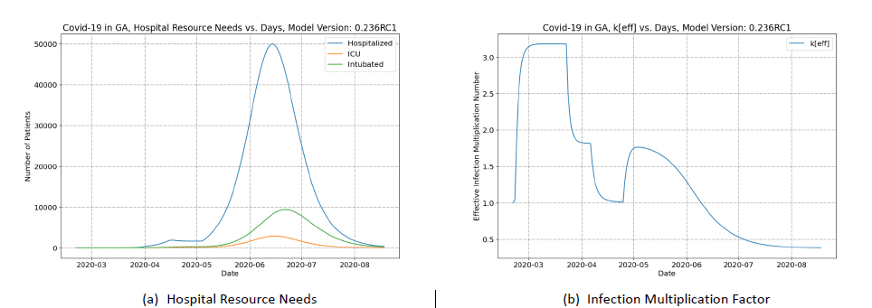
This scenario, admittedly, is pathological. This scenario is highly unlikely to come to fruition because the citizenry of Georgia will surely, in the coming months, maintain social distancing regardless of any relaxation of state-wide social distancing policies. This would imply a persistence of a low contact rate which is not currently part of the SEIR+AQ model. Therefore, while the SEIR+AQ model predicts that GA would have to reimpose some social distancing measures in mid-May to counteract hospital crowding – the continued practice of voluntary social distancing by Georgians will likely delay the date when such orders would be necessary.
An area of future work would be to implement a feature in the code to allow a staggered reopening process that would allow the contact rate to increase slowly over time when social distancing orders are relaxed or revoked.
The results of these calculations, nonetheless, show that there can be significant consequences to reopening businesses and relaxing social distancing measures prematurely; particularly when the mitigation measures have still not been enough to quell the spread of the infection by lowering the infection multiplication factor below one.
Reopening in this case introduces a positive worth of 60¢ and this is such a significant positive worth that the rate of infection increases dramatically and there is a rather rapid depletion effect. The results show that the keff drops below 0.5 by the end of July – indicating a large proportion of the population has recovered from the infection and herd immunity is achieved.
Discussion
This paper has described a simple model for predicting the spread of SARS-CoV-2 and the resulting consequences in terms of hospital system burden and virus-caused fatalities. The SEIR+AQ model has been exercised for several states in the US and the results show reasonable agreement with available data and the predictions of another leading COVID-19 model (the IHME model).
The SEIR+AQ model calculates the infection multiplication factor, which is a concept very similar to the viral reproduction number and examples were presented to demonstrate how the calculated infection multiplication factor can be used as a way to quantify the effectiveness, or the worth, of different mitigation and containment strategies as implemented through public policies. This quantification would allow hypothetical policymakers to evaluate portfolios of mitigation and containment strategies to ensure that the combination of policies do enough to suppress the spread of the virus.
Scenario predictions were presented with different reopening strategies to demonstrate viability of reopening under specific conditions (low infection multiplication number) with containment strategies and how enhancing or augmenting certain strategies even by a small amount can substantially reduce virus fatalities and hospitalizations. Predictions were made for reopening scenarios without containment and the predicted results were extreme in terms of consequences. It is worth noting that the forecast from this model is very conservative in that it does not account for contact rates remaining lower than normal even after social distancing measures are relaxed and therefore overpredicts peak hospital resource needs and casualties.
Throughout this paper, several areas of future work have been mentioned, the below sections summarize these future work recommendations and add a few others.
Sensitivity and uncertainty analysis
The uncertainty in the SEIR+AQ model has not been evaluated, and this severely limits the usefulness of the model in policy decision making. An area of future work would be to perform additional integral assessment and meta-analysis to establish ranges for the various parameters in the model. A Wilks based approach11,12 could then be used to determine an appropriate number of Monte Carlo trials necessary to determine some one-sided upper tolerance limit value of the key figures of merit. Since the figures of merit are all dependent, a one-sided upper tolerance limit result could be achieved using Monte Carlo techniques with a small number of trials (< 100). Since this could be automated in a computer code, the results would remain accessible and could be generated on a personal computer without trouble.
Expanded verification and validation
The verification and validation of the SEIR+AQ could, and should, be expanded as an area of future work. There are many states and counties listed in the www.covidtracking.com databases13 that could form the basis for expanded validation of the SEIR+AQ model. In addition, there are other COVID-19 modeling efforts apart from IHME where the SEIR+AQ model results could be compared and this should be pursued.
Policy compliance
In many of the mitigation and containment strategies, the model relies on simulating the compliance of citizens with the policies according to certain user-specified factions. For example, f tracks the fraction wearing masks and TMC represents the fraction that would honor a quarantine order. These compliance fractions are conjectural at the current time and experience in containing the outbreak in reopened states will proceed without the data or experience to better quantify these parameters. An area of future work should be to better enumerate the compliance fractions.
Medical care seeking as a cultural parameter and hospital discharge rate
Hospitalization predictions could likely be improved by reimagining the parameter κ. Currently, hospitalizations are assumed to occur in the model according to severity of symptoms. However, in the US, additional factors are likely to influence whether an infected individual will seek medical attention beyond just the severity of the symptoms (see 14). Supply chain issues, such as availability of personal protective equipment, will affect the availability of medical care in the US, but the availability already varies dramatically from region to region in the US. Many residents in rural areas of the US may be a far distance from the nearest hospital, which will be a factor in whether these residents seek such medical care. Furthermore, insurance coverage varies greatly from state to state in the US; so ability to pay will also be a factor in the hospitalization and discharge rates. An area of future work could use model fitting procedures or algorithms to study potential variations in κ across different states in the US and perhaps correlate κ with other factors (e.g., supply chain issues, distances to hospitals, and the rate of insurance coverage) which may have a significant impact on the likelihood of infected individuals to seek medical treatment in hospitals. Similar approaches could be used to better quantify the hospital discharge rate.
Assessment of containment strategy models
Modeling parameters for the containment strategies currently implemented are largely conjectural and cannot be relied upon to make accurate predictions until there is a means of assessing the model performance. This will be an area of future work to validate containment models against states that implement those policies in the coming months.
Modeling widespread diagnostic and serological testing access
The current SEIR+AQ model does not consider the ramifications of wide-spread access to diagnostic or serological testing. However, should testing become widely accessible the model predictions in terms of the number of cases would no longer be accurate moving forward because these tests would no longer be rationed according to symptom severity. Therefore, to perform future validation of the model against data in a regime where diagnostic and serological testing is widely accessible would require rethinking the current approach to predict the number of cases.
A more detailed model of testing may also assist in understanding differences between the SEIR+AQ model predictions for Michigan and the available data.
Modeling staggered reopening strategies
The current model has the flexibility to impose and revoke a social distancing order, but a staggered implementation of social distancing measures or a staggered relaxation of social distancing is not possible in the current code structure. Using Washington, DC as an example, schools were closed before non-essential businesses were closed – so the social distancing orders were imposed in a staggered manner. Social distancing orders will most likely be lifted in a staggered manner as well. For example, retail businesses may be allowed to re-open for restaurants. This type of staggered relaxation of social distancing orders cannot be modeled in the current code.
An area of future work is to allow such staggered approaches. This could be implemented in the code by use a mobility factor. Each step in the staggered policy implementation might reduce the contact rate by a mobility reduction factor or by a fixed mobility reduction amount. The exact implementation would be in the scope of future work. However, by having the flexibility to define a series of policies with variable effects on the contact rate, this series could then be applied or revoked in a staggered manner. This would more closely match the reality of how social distancing measures were imposed and the likely process by which they will be relaxed in the US.
Automatic fitting of cultural parameters to validation datasets
The current validation involved comparison of the model to state-by-state data, but some cultural parameters were tuned to achieve good agreement between the model and data. In the current work these parameters were tuned manually. This process could easily be automated. An automated process could examine a wider scope of cultural parameters, ranges could be imposed on each parameter, and then a genetic algorithm could be used to randomly vary the parameters in a set and compute the performance of each set against a utility function. The utility function would just be, for example, the root-mean-square difference between the cases and casualties. The genetic algorithm would randomly mutate the cultural parameters in the set based on the “fitness” of each set relative to the utility function until the process automatically generates a set of cultural parameters that most closely replicates the available data.
Use of a genetic algorithm in this case can lead to overfitting of the data and must be exercised with caution. Once such a method has been developed, results must undergo a comprehensive study to ensure the performance does not overfit the parameters leading to invalid predictions. A method for studying the performance of the algorithm might consider cross-comparison of results from different states. The differences in the genetic algorithm results from state to state could be studied in light of other data (e.g., comorbidity prevalence, mobility data, insurance coverage, etc.) to ensure the differences are reasonable.
Nation modeling
The current model is simple and models the progression of the outbreak through a population assuming a uniform mixing of the population by virtue of how contacts leading to exposure are mathematically treated. This tends to be a poor approximation for nations where there is some distance and separation between major population centers. This is compensated in the model by using a low average contact rate. An alternative modeling approach for nations would be to assemble models for individual metropolitan areas and model the interaction between these metropolitan areas in a network (i.e., a series of vertices connected by edges in a graph).
A similar concept for modeling infection spread has been proposed15 but here the uniform mixing assumption would remain for cities which would serve as vertices in the graph. The vertices could then transfer population along edges in the graph. To model an entire nation this may require modeling ~100-1,000 cities as vertices and linking each SEIR+AQ model with edges. The treatment of population flow along the edges would be relatively simple to implement in the model. Since the SEIR+AQ model is simple, a large network may be feasibly simulated on a personal computer.
Accounting for seasonality
SARS-CoV-2 transmission may be sensitive to the weather.16,17 The model could likely be improved by implementing a time dependent transmission probability (β) where the transmission can vary depending on the season. The seasonal variation in transmission probability can have significant implications for the predictive capability of models over long periods (i.e., longer than a single season). Data from opposing hemispheres can be used to fit the transmission probability in the southern hemisphere (for instance) and then apply that transmission probability in the next season in the northern hemisphere and vice-versa.
Possibilities for novel treatment
The experimental drug remdesivir might be a viable treatment for COVID-19 to reduce recovery time.18,19 The development and adoption of a novel treatment can be captured in the model by implementing a feature that allows the recovery rate to be updated during the simulation.
CONCLUSIONS
Using historical data to first tune a SEIR+AQ model gives confidence in the calculation of the respective worth of the control measures, which can then aid in the assessment of different policy options moving forward in the US. When evaluating the effectiveness of mitigation measures, the combined worth can be compared to the necessary worth of -1$ and adjusted to meet the need. If a mitigation measure might be relaxed, it may be compensated by a containment strategy of a comparable worth. The methods demonstrated in this paper can aid US policymakers in designing an appropriate portfolio of measures for their state.
Acknowledgements: The author would like to acknowledge Dr. Lisa Mullen and Dr. Whitney Raas for reviewing a draft of this paper and providing valuable feedback.
Declaration: PY is an employee of the United States Nuclear Regulatory Commission (NRC). The current work embodied in this paper was not conducted under the auspices of the NRC of the US Government, was not funded by the NRC of any other organization and was conducted on the author’s personal time. The views expressed herein are solely those of the author and do not necessarily represent the views of the NRC or the United States government.
Funding: None.
Authorships contribution: PY is the sole author.
Competing interests: The author completed the Unified Competing Interest form at www.icmje.org/coi_disclosure.pdf (available upon request from the corresponding author), and declare no conflicts of interest.
Correspondence to:
Dr Peter Yarsky
United States Nuclear Regulatory Commission
Washington, DC 20555-0001
[email protected]